Supplemental Codes for Project 3.
Alfa Heryudono MTH572/472 Numerical PDE
Our goal is to solve several simple PDEs in 2D using method of lines. In particular, we will discretize space with finite difference and advance the resulting system of ODEs in time with simple ODE solver. We will also check the accuracy and stability of the problem.
Contents
2-D Diffusion Equation with extra term.
Suppose we are trying to numerically simulate the following 2-D Diffusion equation in the domain ![$[-1,1] \times [-1,1]$](project3supplementhtml_eq16896893380415760150.png) from
from  until
until 
with boundary conditions at all points (x,y) of east, west, north, and south of boundaries given by the function

and initial condition
Suppose, we want to solve it with 3-point stencil finite-difference in x direction, 3-point stencil finite-difference in y direction (you can call this 5-point stencil if you derive it with 2-D Taylor series), and Forward Euler in time.
- Define sigma
 is ratio
  Hence we define and
  in the beginning of the program and the time step k will be computed by
  from there.
close all; clear all;
format long e % format number in long format
sigma = 2e-1;
- Get 2nd-derivative Differentiation Matrix
a = -1; b = 1;
n = 30; h = (b-a)/(n-1);
one = ones(n,1); % create a column vector of size n by 1 of ones
D2 = spdiags([one -2*one one],[-1 0 1],n,n);
D2(1,1:4) = [2 -5 4 -1]; D2(end,end-3:end) = [-1 4 -5 2]; % Modify first and last row (one-sided weights)
D2 = (1/h^2)*D2; % Don't forget the 1/(h^2) factor
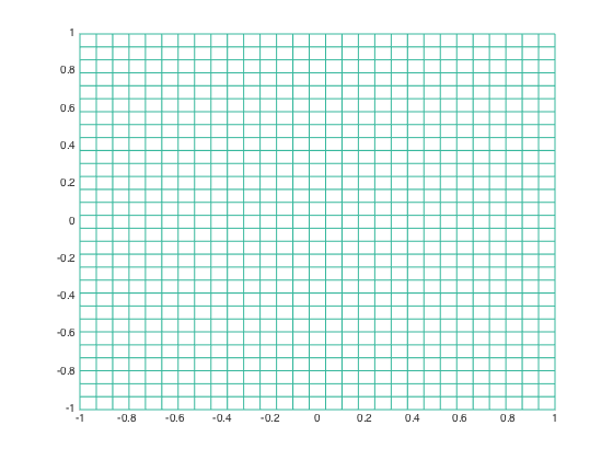
- Create Tensor Product Grid
x = linspace(a,b,n).'; % Create n equally-spaced points in [a,b]
y = x; % set y = x
[X,Y] = meshgrid(x,y);
figure
mesh(X,Y,0*X); view(2); % plot the grid
hold on;
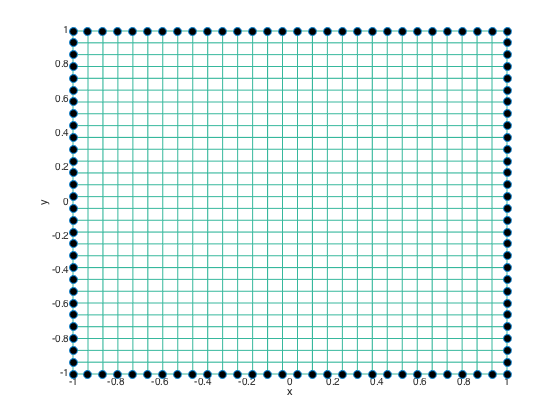
- Flag boundary points and plot them on the grid
flagbdr = true(size(X));
flagbdr(2:end-1,2:end-1) = false; % flag interior points as false
plot(X(flagbdr),Y(flagbdr),'o','MarkerFaceColor','k','MarkerSize',8)
xlabel('x'); ylabel('y');
- Create Laplacian differentiation matrix L = Dxx + Dyy.
I = speye(n); % Create sparse identity matrix
L = kron(D2,I) + kron(I,D2);
- Find indices of boundary points. Strip rows of boundary points and split boundary columns from the main matrix.
bdridx = find(flagbdr(:)); % get the linear indices of boundary nodes
L(bdridx,:) = []; % Strip the boundary rows
BDRCols = L(:,bdridx); % Store the boundary columns
L(:,bdridx) = []; % Strip the boundary columns
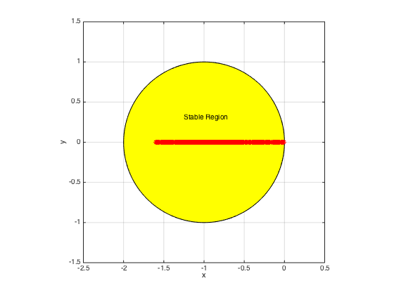
Plot the the eigenvalues scaled with time-step k of the modified operator L.
k = h^2*sigma; % time-step
evscaled = k*eig(full(L));

figure;
z = exp(1i*pi*(0:200)/100); r = z - 1; s = 1; R = r./s;
plot(R); fill(real(R),imag(R),'y'); hold on
plot(real(evscaled),imag(evscaled),'*r')
text(-1.25,0.3,'Stable Region'); xlabel('x'); ylabel('y')
axis([-2.5 0.5 -1.5 1.5]), axis square, grid on
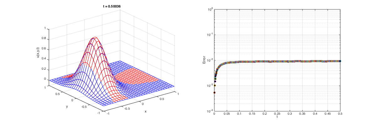
- Define the extra term, boundary condition and initial condition functions. Choose the BC and initial conditions from the exact solution.
uexact = @(x,y,t) exp(-5*(2*(x+sin(t)).^2 + y.^2));
g = uexact;
f = @(x,y,t) -10*(17 + 2*cos(t)*x - 20*cos(2*t) + 80*sin(t)*x + sin(2*t) + 40*x.^2 + 10*y.^2).*exp(-5*(2*(x+sin(t)).^2+y.^2)); % Forcing function
Note that the scaled eigenvalues are in the stability region. Hence, we expect this simulation to be stable. Now let's march the solution in time with Forward Euler.
Tinit = 0; Tfinal = 0.5;
t = Tinit; I = speye(size(L));
u0 = uexact(X,Y,t); % Initial condition
u = u0; u(flagbdr) = g(X(flagbdr),Y(flagbdr),t); % set boundary conditions

% Plot stuff
figure('Position',[100 100 1200 400])
subplot(1,2,1)
graph1 = mesh(X,Y,u0,'EdgeColor','r'); % Plot of numerical solution
hold on
graph2 = mesh(X,Y,u0,'EdgeColor','b'); % Plot of exact solution
t1 = title(sprintf('t = %3.5f',t));
xlim([-1.01 1.01]); ylim([-1.01 1.01]); zlim([-0.1 1.01]);
xlabel('x'); ylabel('y'); zlabel('u(x,y,t)');
subplot(1,2,2)
semilogy(t,NaN,'o','MarkerFacecolor','k'); grid on;
hold on;
xlim([Tinit Tfinal]); ylim([1e-4 1e+0]);
xlabel('t'); ylabel('Error');

u = u(:); u0 = u0(:); X = X(:); Y = Y(:); % vectorize u, u0, X, and Y
while t < Tfinal
    u(~flagbdr) = (I + k*L)*u0(~flagbdr) + k*BDRCols*g(X(flagbdr),Y(flagbdr),t) + k*f(X(~flagbdr),Y(~flagbdr),t);
    t = t + k; u(flagbdr) = g(X(flagbdr),Y(flagbdr),t); % Update time and boundary values.
    set(graph1,'zdata',reshape(u,n,n)); % update the plot
    set(graph2,'zdata',reshape(uexact(X,Y,t),n,n)); % update the exact solution plot
    set(t1,'String',sprintf('t = %3.5f',t));
    drawnow
    subplot(1,2,2)
    semilogy(t,norm(u-uexact(X,Y,t),inf),'o','MarkerFacecolor','k');
    drawnow; % draw the updated plot immediately.
    u0 = u;
end
2-D Wave equation.
Suppose we are trying to numerically simulate the following 2-D Diffusion equation in the domain ![$[-1,1] \times x[-1,1]$](project3supplementhtml_eq02170034040599005952.png) from until
from until 

with boundary conditions at all points (x,y) of east, west, north, and south of boundaries given by the function

and initial conditions

Suppose, we want to solve it with 3-point stencil finite-difference in x direction, 3-point stencil finite-difference in y direction (you can call this 5-point stencil if you derive it with 2-D Taylor series), and Leap Frog in time.
Set the time step.
k = 1e-2;
We can re-use matrices from the previous computations. Use a different initial condition.
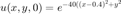
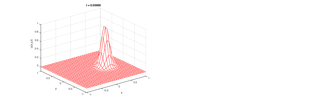
uinit = @(x,y) exp(-40*((x-.4).^2 + y.^2));
u = uinit(X,Y); % Initial condition
u(flagbdr) = 0;
Re-use figure handle from the previous computation and plot the initial condition.
Tinit = 0; Tfinal = 1; t = Tinit;
set(graph1,'zdata',reshape(u,n,n)); set(graph2,'Visible','off');
subplot(1,2,2); set(cla,'Visible','off');
set(t1,'String',sprintf('t = %3.5f',t)); drawnow;
Let us march in time the solution with LeapFrog. We have no exact solution for this.
unew = 0*u; uold = u;
while t < Tfinal
    unew(~flagbdr) = 2*u(~flagbdr) - uold(~flagbdr) + k^2*L*u(~flagbdr);
    t = t + k; % Update time.
    set(graph1,'zdata',reshape(unew,n,n)); % update the plot
    set(t1,'String',sprintf('t = %3.5f',t));
    drawnow; % draw the updated plot immediately.
    uold = u; u = unew;
end
