Lecture 6 (Number 5). Things to do in class

Alfa Heryudono MTH572/472 Numerical PDE

Our goal is to solve a simple ODE on interfal [Tinit,Tfinal]

$u_t = \cos(t)u$

using Forward Euler, Backward Euler, and Trapezoid. We will also check the accuracy of the method.

Set up Exact solution and right hand side function
Forward Euler
Backward Euler
Trapezoid
Redo the problems above with AB3, AM3, and BDF3 in lecture 7.

Set up Exact solution and right hand side function

clear all; close all; format long e
uexact = @(t) exp(sin(t)); % Exact solution to check.
f = @(u,t) cos(t)*u; % RHS function
Tinit = 0; % Starting time
Tfinal = 1; % Final time / Approximate final time.

Forward Euler

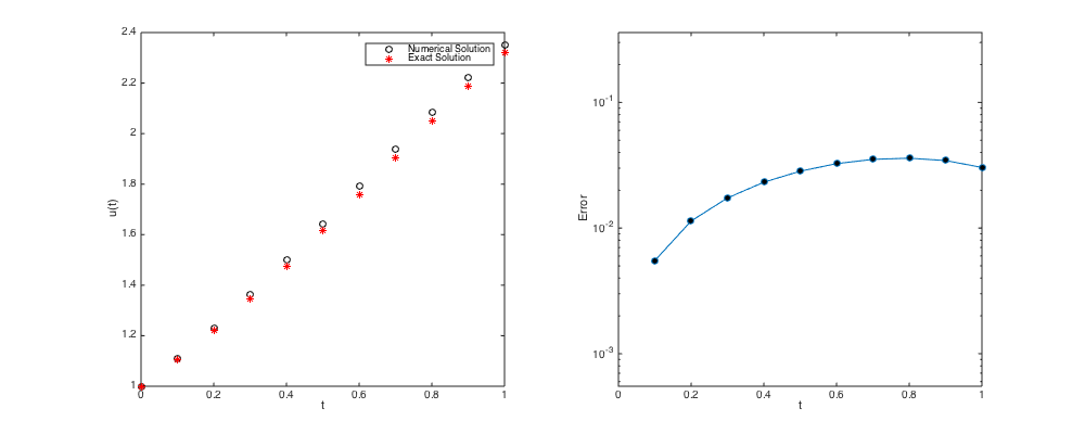
k = 0.1; % Time step.
n = ceil(Tfinal/k); % Round up to the nearest integer if needed.
tn0 = Tinit; un0 = uexact(tn0); % Initial condition taken from exact solution
err = zeros(2,n); % Pre-allocate memory to stores time and error
% Now let's march in time.
figure('Position',[100,100,1000,400]); subplot(1,2,1)
plot(tn0,un0,'ok',tn0,uexact(tn0),'*r'); hold on; % Plot initial condition
legend('Numerical Solution','Exact Solution');
xlabel('t'); ylabel('u(t)');
for i=1:n
    tn1 = tn0 + k;
    un1 = un0 + k*f(un0,tn0);
    plot(tn1,un1,'ok',tn1,uexact(tn1),'*r'); drawnow;
    err(1,i) = tn1; % Store time in the first row of err
    err(2,i) = abs(un1-uexact(tn1)); % Store error in the first row of err.
    un0 = un1; tn0 = tn1;
end
subplot(1,2,2)
semilogy(err(1,:),err(2,:),'-o','markerfacecolor','k');
xlabel('t'); ylabel('Error');
xlim([Tinit Tinit+n*k]); ylim([0.1*min(err(2,:)) 10*max(err(2,:))]);

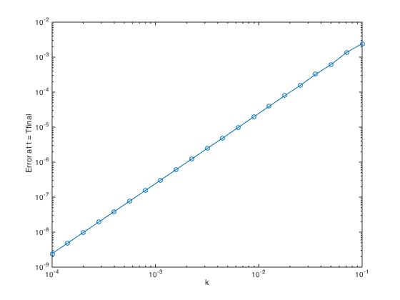
Error accuracy check of Forward Euler at approximately t = Tfinal.

k = logspace(-4,-1,21);
n = ceil(Tfinal./k); err = zeros(1,length(k));
for j=1:length(k)
    tn0 = Tinit; un0 = uexact(tn0);
    for i=1:n(j)
        tn1 = tn0 + k(j);
        un1 = un0 + k(j)*f(un0,tn0);
        un0 = un1; tn0 = tn1;
    end
    err(j) = abs(un1-uexact(tn1));
end
figure
loglog(k,err,'-o')
xlabel('k'); ylabel('Error at t = Tfinal');

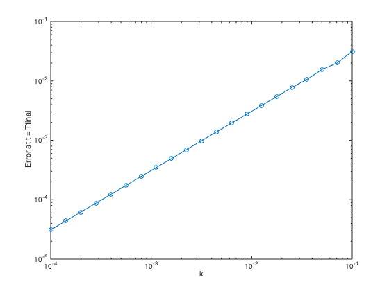
Can you verify the slope of the convergence trend ? is it $\mathcal{O}(k)$ ?

Backward Euler

k = 0.1; % Time step.
n = ceil(Tfinal/k); % Round up to the nearest integer if needed.
tn0 = Tinit; un0 = uexact(tn0); % Initial condition taken from exact solution
err = zeros(2,n); % Pre-allocate memory to stores time and error
% Now let's march in time.
figure('Position',[100,100,1000,400]); subplot(1,2,1)
plot(tn0,un0,'ok',tn0,uexact(tn0),'*r'); hold on; % Plot initial condition
legend('Numerical Solution','Exact Solution');
xlabel('t'); ylabel('u(t)');
for i=1:n
    tn1 = tn0 + k;
    un1 = un0/(1-k*cos(tn1));
    plot(tn1,un1,'ok',tn1,uexact(tn1),'*r'); drawnow;
    err(1,i) = tn1; % Store time in the first row of err
    err(2,i) = abs(un1-uexact(tn1)); % Store error in the first row of err.
    un0 = un1; tn0 = tn1;
end
subplot(1,2,2)
semilogy(err(1,:),err(2,:),'-o','markerfacecolor','k');
xlabel('t'); ylabel('Error');
xlim([Tinit Tinit+n*k]); ylim([0.1*min(err(2,:)) 10*max(err(2,:))]);

Error accuracy check of Backward Euler at t = Tfinal

k = logspace(-4,-1,21);
n = ceil(Tfinal./k); err = zeros(1,length(k));
for j=1:length(k)
    tn0 = Tinit; un0 = uexact(tn0);
    for i=1:n(j)
        tn1 = tn0 + k(j);
        un1 = un0/(1-k(j)*cos(tn1));
        un0 = un1; tn0 = tn1;
    end
    err(j) = abs(un1-uexact(tn1));
end
figure
loglog(k,err,'-o')
xlabel('k'); ylabel('Error at t = Tfinal');

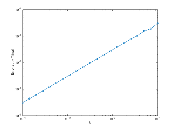
Can you verify the slope of the convergence trend ? is it $\mathcal{O}(k)$ ?

Trapezoid

k = 0.1; % Time step.
n = ceil(Tfinal/k); % Round up to the nearest integer if needed.
tn0 = Tinit; un0 = uexact(tn0); % Initial condition taken from exact solution
err = zeros(2,n); % Pre-allocate memory to stores time and error
% Now let's march in time.
figure('Position',[100,100,1000,400]); subplot(1,2,1)
plot(tn0,un0,'ok',tn0,uexact(tn0),'*r'); hold on; % Plot initial condition
legend('Numerical Solution','Exact Solution');
xlabel('t'); ylabel('u(t)');
for i=1:n
    tn1 = tn0 + k;
    un1 = (un0+0.5*k*f(un0,tn0))/(1-0.5*k*cos(tn1));
    plot(tn1,un1,'ok',tn1,uexact(tn1),'*r'); drawnow;
    err(1,i) = tn1; % Store time in the first row of err
    err(2,i) = abs(un1-uexact(tn1)); % Store error in the first row of err.
    un0 = un1; tn0 = tn1;
end
subplot(1,2,2)
semilogy(err(1,:),err(2,:),'-o','markerfacecolor','k');
xlabel('t'); ylabel('Error');
xlim([Tinit Tinit+n*k]); ylim([0.1*min(err(2,:)) 10*max(err(2,:))]);

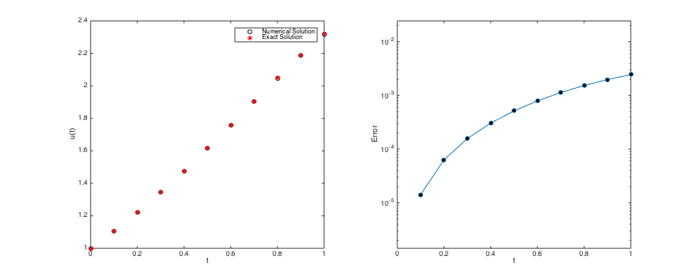
Error accuracy check of Trapezoid at t = Tfinal

k = logspace(-4,-1,21);
n = ceil(Tfinal./k); err = zeros(1,length(k));
for j=1:length(k)
    tn0 = Tinit; un0 = uexact(tn0);
    for i=1:n(j)
        tn1 = tn0 + k(j);
        %un1 = un0/(1-k(j)*cos(tn1));
        un1 = (un0+0.5*k(j)*f(un0,tn0))/(1-0.5*k(j)*cos(tn1));
        un0 = un1; tn0 = tn1;
    end
    err(j) = abs(un1-uexact(tn1));
end
figure
loglog(k,err,'-o')
xlabel('k'); ylabel('Error at t = Tfinal');

Can you verify the slope of the convergence trend ? is it $\mathcal{O}(k^2)$ ?

Redo the problems above with AB3, AM3, and BDF3 in lecture 7.