Lecture 5. Things to do in class.

Alfa Heryudono MTH572/472 Numerical PDE.

Our goal is to solve 1D BVP on interval [a,b]

$u_{xxx} = f(x) \quad x \in (a,b)$

with multiple boundary conditions

$u(a) = g_1, \quad u(b) = g_n, \quad u_x(b) = w_n$

using 3 methods: Row Addition, Ghost Point + Row Replacement, and Ghost Point + Strip Rows + Move Over Columns.

Row Addition Method
Ghost Point + Row Replacement
Ghost Point + Strip Rows and Move Over Columns

Row Addition Method

clear all; close all; % clear all to start fresh
format long e % format number in long format

Define the forcing and boundary condition functions

u = @(x) exp(-x).*sin(pi*x); % Define the BC function (also happens to be the exact solution)
ux = @(x) exp(-x).*(pi*cos(pi*x)-sin(pi*x)); % Define the function for Neumann BC.
f = @(x) exp(-x).*(pi*(3-pi^2)*cos(pi*x) + (3*pi^2-1)*sin(pi*x)); % Forcing function

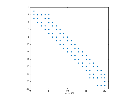
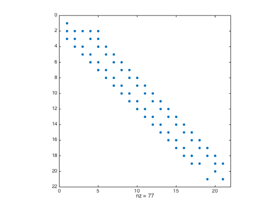
Form the (n+1) x n least-square system.

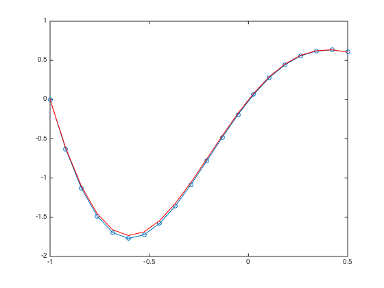
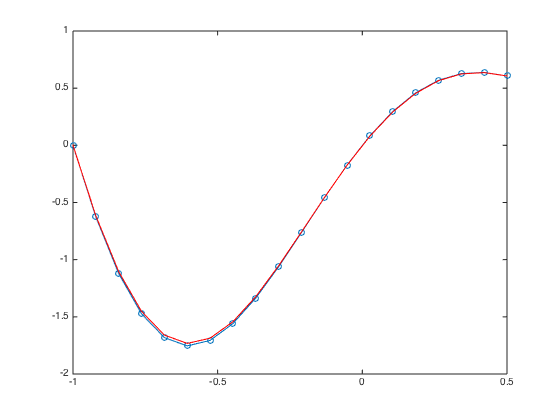
a = -1; b = 0.5; n = 20; h = (b-a)/(n-1);
x = linspace(a,b,n).'; one = ones(n,1);
D3 = spdiags([-0.5*one one -one 0.5*one],[-2 -1 1 2],n,n); % Get 2nd-order 3rd derivative matrix
D3(1,:) = 0; D3(1,1) = 1; % Modify first row (Dirichlet BC at x=a)
D3(2,1:5) = [-1.5 5 -6 3 -0.5]; % Modify the 2nd row (non-centered weights)
D3(n-1,n-4:n) = [0.5 -3 6 -5 1.5]; % Modify the (n-1)th row (non-centered weights)
D3(n,:) = 0; D3(n,n) = 1; % Modify last row (Dirichlet BC at x=b)
D3(n+1,:) = 0; % Add one additional row.
D3(n+1,n-2:n) = [0.5 -2 1.5]; % Modify the additional row (Neumann BC)
F = h^3*[f(x);0]; F(1) = u(a); F(n) = u(b); F(n+1) = h*ux(b); % Modify right hand side
spy(D3) % Plot the structure of the sparse matrix
U = D3\F; % solve the (n+1) x n system. For rectangular system, \ is doing least square.
figure
plot(x,U,'-o',x,u(x),'-r'); % Plot the numerical sol vs exact sol
norm(U-u(x),Inf) % Compute the infinity norm

ans =

     3.695282571570724e-02

Row addition method convergence test without scaling

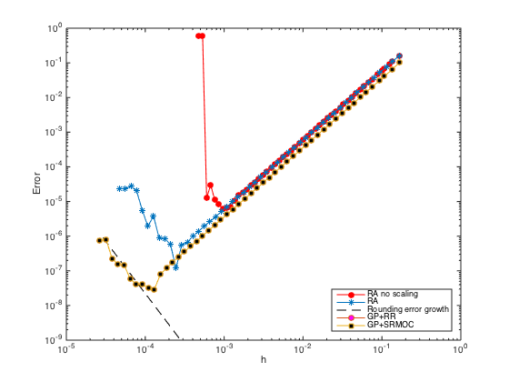
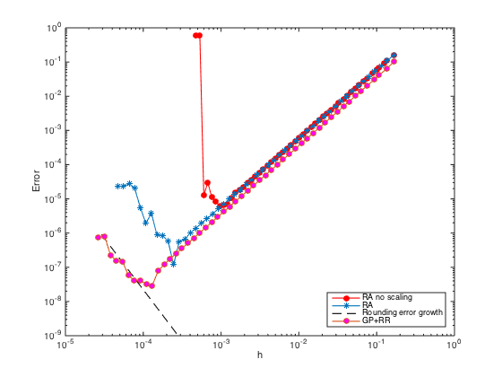
n = ceil(logspace(1,3.5));
h = (b-a)./(n-1);
err = zeros(length(n),1); % Pre-allocate memory to store errors
for i=1:length(n)
    x = linspace(a,b,n(i)).'; one = ones(n(i),1); % create a column vector of size n by 1 of ones
    D3 = spdiags([-0.5*one one -one 0.5*one],[-2 -1 1 2],n(i),n(i)); % Get 2nd-order 3rd derivative matrix
    D3(1,:) = 0; D3(1,1) = h(i)^3; % Modify first row (Dirichlet BC at x=a)
    D3(2,1:5) = [-1.5 5 -6 3 -0.5]; % Modify the 2nd row (non-centered weights)
    D3(n(i)-1,n(i)-4:n(i)) = [0.5 -3 6 -5 1.5]; % Modify the (n-1)th row (non-centered weights)
    D3(n(i),:) = 0; D3(n(i),n(i)) = h(i)^3; % Modify last row (Dirichlet BC at x=b)
    D3(n(i)+1,:) = 0; % Add one additional row.
    D3(n(i)+1,n(i)-2:n(i)) = [0.5 -2 1.5]*h(i)^2; % Modify the additional row (Neumann BC)
    D3 = (1/h(i)^3)*D3;
    F = [f(x);0]; F(1) = u(a); F(n(i)) = u(b); F(n(i)+1) = ux(b); % Modify right hand side
    U = D3\F; % solve the (n+1) x n system. For rectangular system, \ is doing least square.
    err(i) = norm(U-u(x),Inf);
end
figure
loglog(h,err,'-or','markerfacecolor','r') % Plot the errors in logscale
xlabel('h'); ylabel('Error')
legend('RA no scaling','Location','SouthEast')

Warning: Rank deficient, rank = 2811, tol =  1.003378e+00. 
Warning: Rank deficient, rank = 3162, tol =  1.606360e+00.

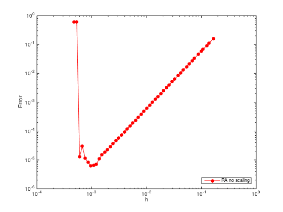
Although the slope of the error convergence is 2 (second order), the rank deficiency issue due to the ill-conditioning of the system for small h prevents the error to go down even further.

Row addition method convergence test with scaling

n = ceil(logspace(1,4.5));
h = (b-a)./(n-1);
err = zeros(length(n),1); % Pre-allocate memory to store errors
for i=1:length(n)
    x = linspace(a,b,n(i)).'; one = ones(n(i),1); % create a column vector of size n by 1 of ones
    D3 = spdiags([-0.5*one one -one 0.5*one],[-2 -1 1 2],n(i),n(i)); % Get 2nd-order 3rd derivative matrix
    D3(1,:) = 0; D3(1,1) = 1; % Modify first row (Dirichlet BC at x=a)
    D3(2,1:5) = [-1.5 5 -6 3 -0.5]; % Modify the 2nd row (non-centered weights)
    D3(n(i)-1,n(i)-4:n(i)) = [0.5 -3 6 -5 1.5]; % Modify the (n-1)th row (non-centered weights)
    D3(n(i),:) = 0; D3(n(i),n(i)) = 1; % Modify last row (Dirichlet BC at x=b)
    D3(n(i)+1,:) = 0; % Add one additional row.
    D3(n(i)+1,n(i)-2:n(i)) = [0.5 -2 1.5]; % Modify the additional row (Neumann BC)
    F = h(i)^3*[f(x);0]; F(1) = u(a); F(n(i)) = u(b); F(n(i)+1) = h(i)*ux(b); % Modify right hand side
    U = D3\F; % solve the (n+1) x n system. For rectangular system, \ is doing least square.
    err(i) = norm(U-u(x),Inf);
end
figure(3)
hold on;
loglog(h,err,'-*','markerfacecolor','b') % Plot the errors in logscale
xlabel('h'); ylabel('Error')

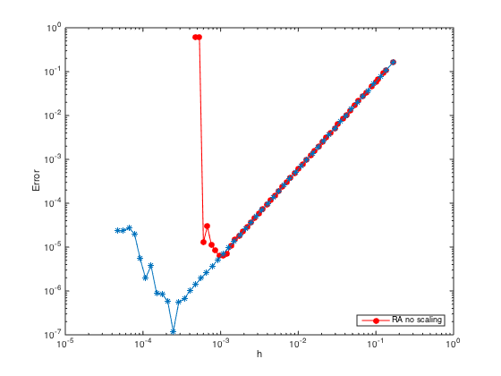
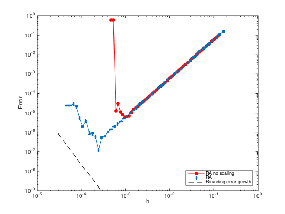
With scaling, the ill-conditioning issue can be remedied. The error can go down further until the rounding error kicks in with growth of order

$\displaystyle \mathcal{O}\left(\frac{\varepsilon}{h^3}\right)$

where $\varepsilon$ is the machine precision.

n = ceil(logspace(3.75,4.75)); h = (b-a)./(n-1); loglog(h,1e-4*eps./h.^3,'--k')
legend('RA no scaling','RA','Rounding error growth','Location','SouthEast')

Ghost Point + Row Replacement

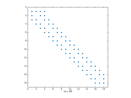
Form the (n+1) x (n+1) square system.

a = -1; b = 0.5; n = 20; h = (b-a)/(n-1);
x = linspace(a,b,n).';
x = [x;x(end)+h]; % Add a ghost point
one = ones(n+1,1); % create a column vector of size n+1 by 1 of ones
D3 = spdiags([-0.5*one one -one 0.5*one],[-2 -1 1 2],n+1,n+1); % Get 2nd-order 3rd derivative matrix
D3(1,:) = 0; D3(1,1) = 1; % Modify first row (Dirichlet BC at x=a)
D3(2,1:5) = [-1.5 5 -6 3 -0.5]; % Modify the 2nd row (non-centered weights)
D3(n,:) = 0; D3(n,n) = 1; % Modify n-th row (Dirichlet BC at x=b)
D3(n+1,n-1:n+1) = [-0.5 0 0.5]; % Modify the row of ghost point (Neumann BC)
figure
spy(D3) % Plot the structure of the sparse matrix
F = h^3*f(x); F(1) = u(a); F(n) = u(b); F(n+1) = h*ux(b); % Modify right hand side
U = D3\F; % solve the (n+1) x (n+1) system.
figure
plot(x(1:n),U(1:n),'-o',x(1:n),u(x(1:n)),'-r'); % Plot the numerical sol vs exact sol
norm(U(1:n)-u(x(1:n)),Inf) % Compute the infinity norm (excluding value at ghost point)

ans =

     2.240588682198541e-02

Ghost Point + Row Replacement convergence test with scaling.

n = ceil(logspace(1,4.75));
h = (b-a)./(n-1);
err = zeros(length(n),1); % Pre-allocate memory to store errors
for i=1:length(n)
    x = linspace(a,b,n(i)).'; x = [x;x(end)+h(i)]; % Add a fictitious point
    one = ones(n(i)+1,1); % create a column vector of size n+1 by 1 of ones
    D3 = spdiags([-0.5*one one -one 0.5*one],[-2 -1 1 2],n(i)+1,n(i)+1); % Get 2nd-order 3rd derivative matrix
    D3(1,:) = 0; D3(1,1) = 1; % Modify first row (Dirichlet BC at x=a)
    D3(2,1:5) = [-1.5 5 -6 3 -0.5]; % Modify the 2nd row (non-centered weights)
    D3(n(i),:) = 0; D3(n(i),n(i)) = 1; % Modify n-th row (Dirichlet BC at x=b)
    D3(n(i)+1,n(i)-1:n(i)+1) = [-0.5 0 0.5]; % Modify the row of ghost point (Neumann BC)
    F = h(i)^3*f(x); F(1) = u(a); F(n(i)) = u(b); F(n(i)+1) = h(i)*ux(b); % Modify right hand side
    U = D3\F; % solve the (n+1) x (n+1) system.
    err(i) = norm(U(1:n(i))-u(x(1:n(i))),Inf); % Compute the infinity norm (excluding value at ghost point)
end
figure(3); hold on;
loglog(h,err,'-o','markerfacecolor','m') % Plot the errors in logscale
xlabel('h'); ylabel('Error')
legend('RA no scaling','RA','Rounding error growth','GP+RR','Location','SouthEast')

Ghost Point + Strip Rows and Move Over Columns

Form the reduced square system matrix

a = -1; b = 0.5; n = 20; h = (b-a)/(n-1);
x = linspace(a,b,n).';
x = [x;x(end)+h]; % Add a fictitious point
one = ones(n+1,1);
D3 = spdiags([-0.5*one one -one 0.5*one],[-2 -1 1 2],n+1,n+1); % Get 2nd-order 3rd derivative matrix
D3(2,1:5) = [-1.5 5 -6 3 -0.5]; % Modify the 2nd row (non-centered weights)
D3([1 n n+1],:) = []; % Strip rows 1, n, and n+1
F = f(x); F = h^3*F; F([1 n n+1]) = []; % Pre-allocate the RHS
F = F - u(a)*D3(:,1) - u(b)*D3(:,n) - 2*h*ux(b)*D3(:,n+1); % Modify RHS.
D3(:,[1 n n+1]) = []; % Strip columns 1, n, and n+1
D3(n-2,n-2) = 0.5; % Modify the entry at (n-2,n-2)
figure
spy(D3) % Plot the structure of the sparse matrix
U = zeros(n,1); U(1) = u(a); U(n) = u(b); % Pre-allocate memory for the solution
U(2:n-1) = D3\F; % solve the (n-2) x (n-2) system.
figure
plot(x(1:n),U,'-o',x(1:n),u(x(1:n)),'-r'); % Plot the numerical sol vs exact sol
norm(U-u(x(1:n)),Inf) % Compute the infinity norm

ans =

     2.240588682198474e-02

Ghost Point + Strip-Rows Move Over Columns convergence test with scaling

n = ceil(logspace(1,4.75));
h = (b-a)./(n-1);
err = zeros(length(n),1); % Pre-allocate memory to store errors
for i=1:length(n)
    x = linspace(a,b,n(i)).';
    x = [x;x(end)+h(i)]; % Add a fictitious point
    one = ones(n(i)+1,1); % create a column vector of size n+1 by 1 of ones
    D3 = spdiags([-0.5*one one -one 0.5*one],[-2 -1 1 2],n(i)+1,n(i)+1); % Get 2nd-order 3rd derivative matrix
    D3(2,1:5) = [-1.5 5 -6 3 -0.5]; % Modify the 2nd row (non-centered weights)
    D3([1 n(i) n(i)+1],:) = []; % Strip rows 1, n, and n+1
    F = f(x); F = h(i)^3*F; F([1 n(i) n(i)+1]) = []; % Pre-allocate the RHS
    F = F - u(a)*D3(:,1) - u(b)*D3(:,n(i)) - 2*h(i)*ux(b)*D3(:,n(i)+1); % Modify RHS.
    D3(:,[1 n(i) n(i)+1]) = []; % Strip columns 1, n, and n+1
    D3(n(i)-2,n(i)-2) = 0.5; % Modify the entry at (n-2,n-2)
    U = zeros(n(i),1); U(1) = u(a); U(n(i)) = u(b); % Pre-allocate memory for the solution
    U(2:n(i)-1) = D3\F; % solve the (n-2) x (n-2) system.
    err(i) = norm(U-u(x(1:n(i))),Inf);
end
figure(3); hold on;
loglog(h,err,'-s','markerfacecolor','k') % Plot the errors in logscale
xlabel('h'); ylabel('Error')
legend('RA no scaling','RA','Rounding error growth','GP+RR','GP+SRMOC','Location','SouthEast')

Lecture 5. Things to do in class.

Contents

Row Addition Method

Ghost Point + Row Replacement

Ghost Point + Strip Rows and Move Over Columns