Lecture 4. Things to do in class.
Our goal is to solve  on the domain
 ![$[-1,1] \times [-1,1]$](mth572lecture4_eq16896893380415760150.png) of the 2D Poisson Equation
of the 2D Poisson Equation

in  , where

and

at the boundaries.
Contents
Number 1
- Get 1D version of 2nd-order 2nd-derivative differentiation matrix. For this particular problem, since
 and
and  , we can use the same 1D 2nd-derivative differentiation matrix, i.e Dxx = Dyy = D2. Watch out for "un-centered" stencil weights.
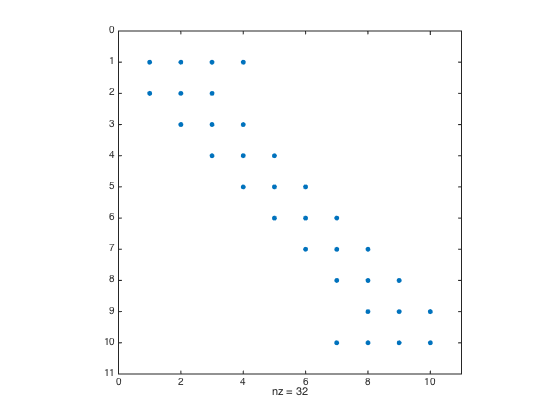
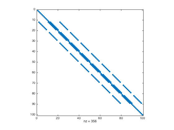
clear all; close all; % clear all to start fresh
format long e % format number in long format
a = -1; b = 1;
n = 10; h = (b-a)/(n-1);
one = ones(n,1); % create a column vector of size n by 1 of ones
D2 = spdiags([one -2*one one],[-1 0 1],n,n);
D2(1,1:4) = [2 -5 4 -1]; D2(end,end-3:end) = [-1 4 -5 2]; % Modify first and last row (one-sided weights)
D2 = (1/h^2)*D2; % Don't forget the 1/(h^2) factor
spy(D2) % Plot the structure of the sparse matrix
- Create Tensor Product Grid
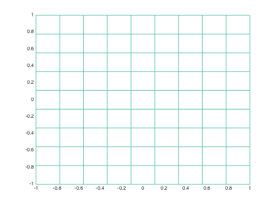
x = linspace(a,b,n).'; % Create n equally-spaced points in [a,b]
y = x; % set y = x
[X,Y] = meshgrid(x,y);
figure
mesh(X,Y,0*X); view(2); % plot the grid
hold on;
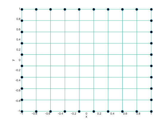
- Flag boundary points and plot them on the grid
flagbdr = true(size(X));
flagbdr(2:end-1,2:end-1) = false; % flag interior points as false
plot(X(flagbdr),Y(flagbdr),'o','MarkerFaceColor','k','MarkerSize',8)
xlabel('x'); ylabel('y');
- Define the forcing and boundary condition functions and their discrete values
u = @(x,y) exp(-(x.^2+0.5*y.^2)); % Define the BC function (also happens to be the exact solution)
f = @(x,y) -(4*x.^2 + y.^2 - 3).*exp(-(x.^2 +0.5*y.^2)); % Forcing function
F = f(X,Y);
F(flagbdr) = u(X(flagbdr),Y(flagbdr)); % at boundary nodes, replace rhs values.
F = F(:); % vectorize F
- Create Laplacian differentiation matrix L = Dxx + Dyy.
I = speye(n); % Create sparse identity matrix
L = -(kron(D2,I) + kron(I,D2));
- Modify rows that correspond to boundary conditions (row replacement) and plot the matrix L
bdridx = find(flagbdr(:)); % get the linear indices of boundary nodes
L(bdridx,:) = 0; % Set the boundary rows to zeros
idx = sub2ind(size(L),bdridx,bdridx);
L(idx) = 1; % set 1 to the diagonal entries of boundary rows
figure;
spy(L); % plot L
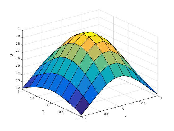
- Solve U and compare with the exact solution
U = L\F;
norm(U-u(X(:),Y(:)),Inf)
U = reshape(U,n,n);
figure
surf(X,Y,U); xlabel('x'); ylabel('y'); zlabel('U');
ans =

     8.733515070539877e-03
Number 2
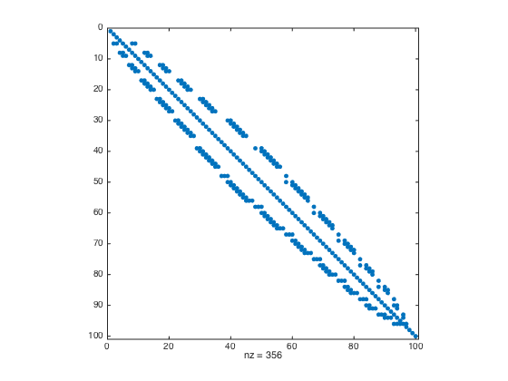
- Perform Cuthill-McKee Permutation to the modified matrix L
P = symrcm(L);
spy(L(P,P))
- Solve U and compare with the exact solution
U = zeros(size(F));
U(P) = L(P,P)\F(P);
norm(U-u(X(:),Y(:)),Inf)
ans =

     8.733515070539877e-03
- Instead of using backslash \, you also use one of the iterative solvers that you learned in numerical linear algebra such as gmres for non symmetric matrix.
U = zeros(size(F));
MAXITER = 20; TOL = 1e-13; RESTART = []; % No restart.
[U(P),FLAG,RELRES,ITER,RESVEC] = gmres(L(P,P),F(P),RESTART,TOL,MAXITER);
norm(U-u(X(:),Y(:)),Inf)
ans =

     8.733515070537212e-03
- Plot the residual convergence of the gmres
semilogy(1:length(RESVEC),RESVEC/norm(F(P)),'-o','markerfacecolor','k','markersize',8);
xlabel('Iteration number');
ylabel('Relative residual');
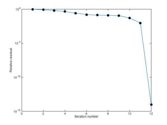
Without restarting, the gmres iteration converges in 12 iterations and the residual suddenly drops from iteration 11 to iteration 12. However, you can also try to pre-condition the matrix L with Incomplete LU decomposition.
U = zeros(size(F));
MAXITER = 20; TOL = 1e-13; RESTART = []; % No restart.
[ML,MU] = ilu(L(P,P),struct('type','ilutp','droptol',1e-6)); % Get the preconditioners.
[U(P),FLAG,RELRES,ITER,RESVEC] = gmres(L(P,P),F(P),RESTART,TOL,MAXITER,ML,MU);
norm(U-u(X(:),Y(:)),Inf)
hold on
semilogy(1:length(RESVEC),RESVEC/norm(F(P)),'-*','markerfacecolor','r','markersize',8);
ans =

     8.733515070539766e-03
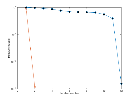
It turns out that the gmres iteration for the pre-conditioned system converges with only 2 iterations. Try to increase the size n to 60 instead of 10.
Number 3
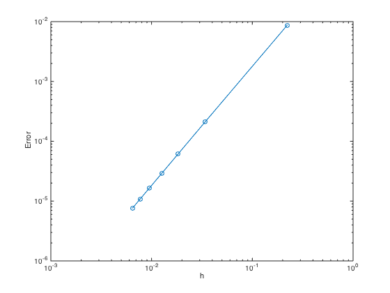
For 2nd order convergence, slope of the error convergence must be 2.
n = 10:50:310; % Create n = 10,110,210,310,...
h = (b-a)./(n-1);
err = zeros(length(n),1); % Pre-allocate memory to store errors
for i=1:length(n)
    one = ones(n(i),1);
    D2 = spdiags([one -2*one one],[-1 0 1],n(i),n(i));
    D2(1,1:4) = [2 -5 4 -1]; D2(end,end-3:end) = [-1 4 -5 2];
    D2 = (1/h(i)^2)*D2;
    x = linspace(a,b,n(i)).';
    y = x; % set y = x
    [X,Y] = meshgrid(x,y);
    flagbdr = true(size(X));
    flagbdr(2:end-1,2:end-1) = false;
    F = f(X,Y); F(flagbdr) = u(X(flagbdr),Y(flagbdr)); F = F(:);
    I = speye(n(i)); L = -(kron(D2,I) + kron(I,D2));
    bdridx = find(flagbdr(:));
    L(bdridx,:) = 0; idx = sub2ind(size(L),bdridx,bdridx); L(idx) = 1;
    U = L\F;
    err(i) = norm(U-u(X(:),Y(:)),Inf);
end
figure
loglog(h,err,'-o') % Plot the errors in logscale
xlabel('h'); ylabel('Error')