Lecture 3. Things to do in class.
Contents
Number 1
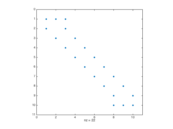
- Get 1D 2nd-order differentiation matrix. For this particular problem, since a=c, b=d, n = m and hx = hy = h, we can use the same 1D differentiation matrix, i.e Dx=Dy=D1.
clear all; close all; % clear all to start fresh
a = -1; b = 1;
n = 10; h = (b-a)/(n-1);
one = ones(n,1); % create a column vector of size n by 1 of ones
D1 = spdiags([-one one],[-1 1],n,n);
D1(1,1:3) = [-3 4 -1]; D1(end,end-2:end) = [1 -4 3]; % Modify first and last row (one-sided weights)
D1 = (0.5/h)*D1; % Don't forget the 1/(2*h) factor
spy(D1) % Plot the structure of the sparse matrix
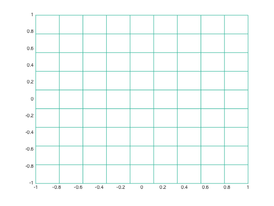
- Create Tensor Product Grid
x = linspace(a,b,n).'; % Create n equally-spaced points in [a,b]
y = x; % set y = x
[X,Y] = meshgrid(x,y);
figure
mesh(X,Y,0*X); view(2); % plot the grid
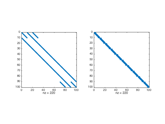
- Create differentiation matrices. Here, I am doing Dx and Dy for you. Can you create the Laplacian operator ?
I = speye(n); % Create sparse identity matrix
Dx = kron(D1,I);
Dy = kron(I,D1);
figure;
subplot(1,2,1); spy(Dx);
subplot(1,2,2); spy(Dy);
Number 2
format long e % format number in long format
u = @(x,y) exp(-(x.^2+0.5*y.^2)); % Define the function
ux = @(x,y) -2*x.*exp(-(x.^2+0.5*y.^2)); % Define the exact u_x of the function
uy = @(x,y) -y.*exp(-(x.^2+0.5*y.^2)); % Define the exact u_y of the function
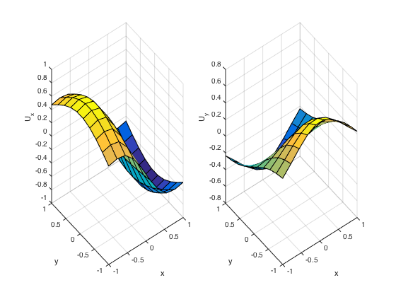
- Compute derivative in matrix way (without kronecker product and without linear indexing). Here I am doing Ux and Uy for you. Can you compute the Laplacian ?
U = u(X,Y); % Function values at nodes
Ux = U*D1.'; % U_x = U*transpose(D)
Uy = D1*U; % U_y = D*U
norm(Ux(:)-ux(X(:),Y(:)),Inf)
norm(Uy(:)-uy(X(:),Y(:)),Inf)
figure
subplot(1,2,1); surf(X,Y,Ux); xlabel('x'); ylabel('y'); zlabel('U_x');
subplot(1,2,2); surf(X,Y,Uy); xlabel('x'); ylabel('y'); zlabel('U_y');
ans =

     4.326197654789388e-02


ans =

     2.179530238274729e-02
- Compute derivatives with kronecker product way and with linear indexing.
Ux = Dx*U(:);
Uy = Dy*U(:);
norm(Ux-ux(X(:),Y(:)),Inf)
norm(Uy-uy(X(:),Y(:)),Inf)
ans =

     4.326197654789388e-02


ans =

     2.179530238274729e-02
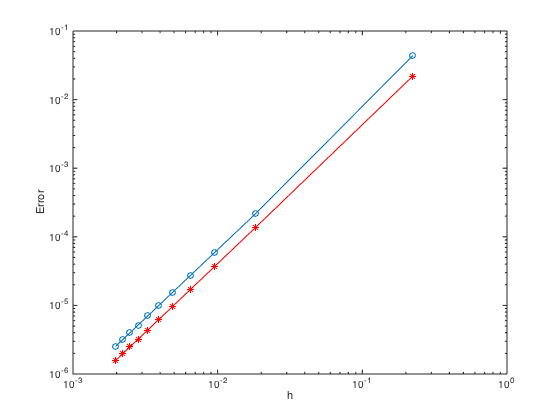
Number 3
For 2nd order convergence, slope must be 2.
n = 10:100:1100; % Create n = 10,110,210,310,...
h = (b-a)./(n-1);
err = zeros(length(n),2); % Pre-allocate memory to store errors
for i=1:length(n)
    one = ones(n(i),1);
    D1 = spdiags([-one one],[-1 1],n(i),n(i));
    D1(1,1:3) = [-3 4 -1]; D1(end,end-2:end) = [1 -4 3];
    D1 = (0.5/h(i))*D1;
    x = linspace(a,b,n(i)).';
    y = x; % set y = x
    [X,Y] = meshgrid(x,y);
    U = u(X,Y); % Function values at nodes
    Ux = U*D1.'; % U_x = U*transpose(D)
    Uy = D1*U; % U_y = D*U
    err(i,1) = norm(Ux(:)-ux(X(:),Y(:)),Inf); % Store err of ux in 1st col
    err(i,2) = norm(Uy(:)-uy(X(:),Y(:)),Inf); % Store err of uy in 2nd col
end
figure
loglog(h,err(:,1),'-o',h,err(:,2),'-*r') % Plot the errors in logscale
xlabel('h'); ylabel('Error')
Number 4
Please do it yourself. Should be easy if you understand and did (1)-(3) correctly.