Lecture 3.5. Things to do in class.
We are testing the error accuracy of the 2D 2nd-order 2nd derivative differentiation matrices. Basically, we are redoing the last page of Lecture 3 with the 2D 2nd derivative differentiation matrices.
Contents
Number 1
- Get the 1D version of 2nd-order 2nd-derivative differentiation matrix. For this particular problem, since a = c, b = d, n = m and h_x = h_y = h, we can use the same 1D 2nd-derivative differentiation matrix, i.e Dxx = Dyy = D2. Please watch out for the ``un-centered'' stencil weights. You need 4 nodes for the un-centered stencils to keep the accuracy of 2nd order.
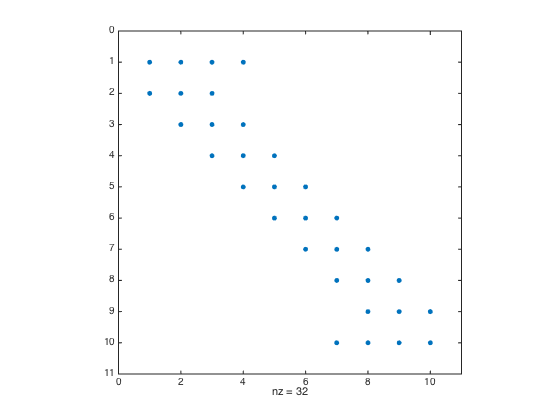
clear all; close all; % clear all to start fresh
a = -1; b = 1;
n = 10; h = (b-a)/(n-1);
one = ones(n,1); % create a column vector of size n by 1 of ones
D2 = spdiags([one -2*one one],[-1 0 1],n,n);
D2(1,1:4) = [2 -5 4 -1]; D2(end,end-3:end) = [-1 4 -5 2]; % Modify first and last row (one-sided weights)
D2 = (1/h^2)*D2; % Don't forget the 1/(h^2) factor
spy(D2) % Plot the structure of the sparse matrix
- Create Tensor Product Grid
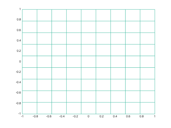
x = linspace(a,b,n).'; % Create n equally-spaced points in [a,b]
y = x; % set y = x
[X,Y] = meshgrid(x,y);
figure
mesh(X,Y,0*X); view(2); % plot the grid
- Create differentiation matrices Dxx and Dyy.
I = speye(n); % Create sparse identity matrix
Dxx = kron(D2,I);
Dyy = kron(I,D2);
figure;
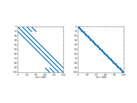
subplot(1,2,1); spy(Dxx);
subplot(1,2,2); spy(Dyy);
Number 2
format long e % format number in long format
u = @(x,y) exp(-(x.^2+0.5*y.^2)); % Define the function
uxx = @(x,y) 2*exp(-(x.^2+0.5*y.^2)).*(2*x.^2 - 1); % Define the exact u_xx of the function
uyy = @(x,y) exp(-(x.^2+0.5*y.^2)).*(y.^2-1); % Define the exact u_yy of the function
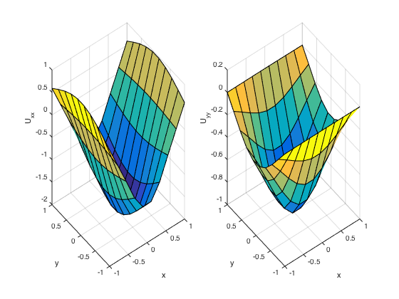
- Compute derivatives Uxx and Uyy without kronecker product and without linear indexing.
U = u(X,Y); % Function values at nodes
Uxx = U*D2.'; % U_x = U*transpose(D)
Uyy = D2*U; % U_y = D*U
norm(Uxx(:)-uxx(X(:),Y(:)),Inf)
norm(Uyy(:)-uyy(X(:),Y(:)),Inf)
figure
subplot(1,2,1); surf(X,Y,Uxx); xlabel('x'); ylabel('y'); zlabel('U_{xx}');
subplot(1,2,2); surf(X,Y,Uyy); xlabel('x'); ylabel('y'); zlabel('U_{yy}');
ans =

     2.378780537064675e-01


ans =

     1.172505202572083e-02
- Compute derivatives Uxx and Uyy with kronecker product and with linear indexing.
Uxx = Dxx*U(:);
Uyy = Dyy*U(:);
norm(Uxx-uxx(X(:),Y(:)),Inf)
norm(Uyy-uyy(X(:),Y(:)),Inf)
ans =

     2.378780537064675e-01


ans =

     1.172505202572083e-02
Number 3
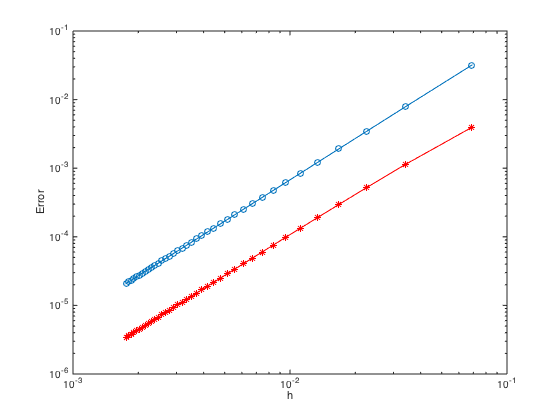
For 2nd order convergence, the error convergence trend slope must be 2.
n = 30:30:1140; % Create n = 10,110,210,310,...
h = (b-a)./(n-1);
err = zeros(length(n),2); % Pre-allocate memory to store errors
for i=1:length(n)
    one = ones(n(i),1);
    D2 = spdiags([one -2*one one],[-1 0 1],n(i),n(i));
    D2(1,1:4) = [2 -5 4 -1]; D2(end,end-3:end) = [-1 4 -5 2]; % Modify first and last row (one-sided weights)
    D2 = (1/h(i)^2)*D2; % Don't forget the 1/(h^2) factor
    x = linspace(a,b,n(i)).';
    y = x; % set y = x
    [X,Y] = meshgrid(x,y);
    U = u(X,Y); % Function values at nodes
    Uxx = U*D2.'; % U_xx = U*transpose(D2)
    Uyy = D2*U; % U_yy = D2*U
    err(i,1) = norm(Uxx(:)-uxx(X(:),Y(:)),Inf); % Store err of ux in 1st col
    err(i,2) = norm(Uyy(:)-uyy(X(:),Y(:)),Inf); % Store err of uy in 2nd col
end
figure
loglog(h,err(:,1),'-o',h,err(:,2),'-*r') % Plot the errors in logscale
xlabel('h'); ylabel('Error')
Additional Problem
Can you redo problem (1)-(3) for the case of mixed derivatives Uxy and/or Uyx ?