Lecture2. Things to do in class.
Contents
Testing 2nd order derivative with problems (1)-(3) from Lecture 1
- Redo Number 1 in Lecture 1 with 2nd-order differentiation matrix
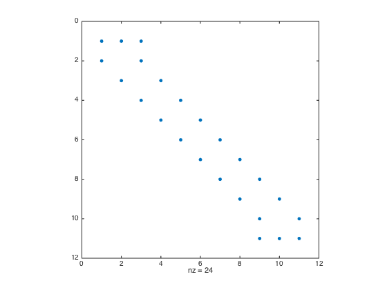
clear all; close all; % clear all to start fresh
% Note: n equal spacing means n+1 points
% as an example let use use a = -1 and b = 1
a = -1; b = 1;
n = 10; h = (b-a)/n;
one = ones(n+1,1); % create a column vector of size n+1 by 1 of ones
D = spdiags([-one one],[-1 1],n+1,n+1);
D(1,1:3) = [-3 4 -1]; D(end,end-2:end) = [1 -4 3]; % Modify first and last row (one-sided weights)
D = (0.5/h)*D; % Don't forget the 1/(2*h) factor
spy(D) % Plot the structure of the sparse matrix
- Redo Number 2 in Lecture 1 with 2nd-order differentiation matrix
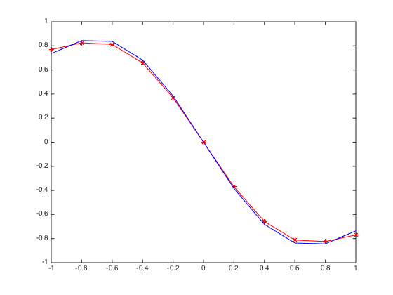
format long e % format number in long format
u = @(x) exp(-x.^2); % Define the function
ux = @(x) -2*x.*exp(-x.^2); % Define the exact derivative of the function
x = linspace(a,b,n+1).'; % Create n+1 equally-spaced points in [a,b]
uux = D*u(x); % Compute numerical derivative
err = norm(uux-ux(x),Inf) % Compute infnorm (u'_num - u'_exact)
figure
plot(x,uux,'-*r',x,ux(x),'-b')
err =

     3.387873412420639e-02
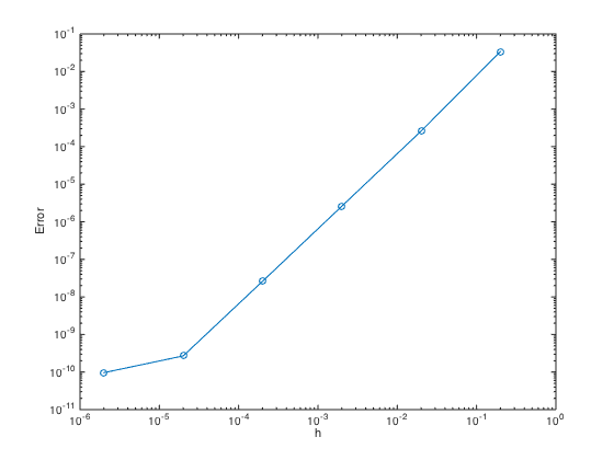
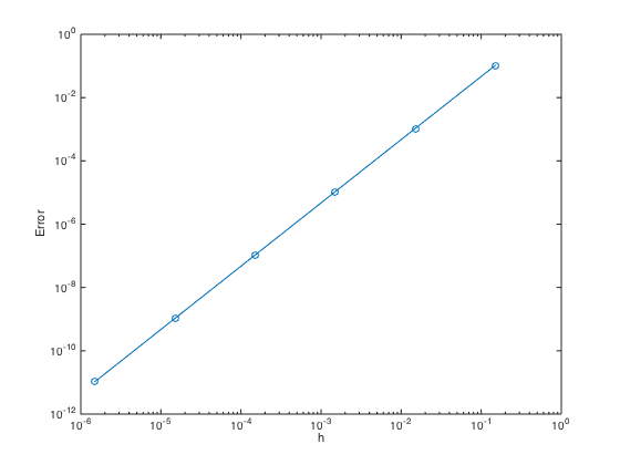
- Redo Number 3 in Lecture 1 with 2nd-order differentiation matrix Can you check what is the slope of the error convergence ? Any idea why the error is somewhat level off when h is getting smaller ?
n = 10.^(1:6); % Create n = 10,100,1000,10000,...
h = (b-a)./n;
err = zeros(length(n),1); % Pre-allocate memory to store errors
for i=1:length(n)
    one = ones(n(i)+1,1);
    x = linspace(a,b,n(i)+1).';
    D = spdiags([-one one],[-1 1],n(i)+1,n(i)+1);
    D(1,1:3) = [-3 4 -1]; D(end,end-2:end) = [1 -4 3]; D = (0.5/h(i))*D;
    uux = D*u(x);
    err(i) = norm(uux-ux(x),Inf);
end
figure
loglog(h,err,'-o') % Plot the error in logscale
xlabel('h'); ylabel('Error')
Number 1
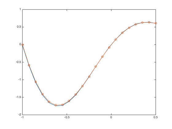
a = -1; b = 0.5;
n = 20; h = (b-a)/n;
x = linspace(a,b,n+1).';
gn = exp(-0.5); % boundary condition at x=0.5
f = @(x) (pi*cos(pi*x)-sin(pi*x)).*exp(-x); % Right hand side function
one = ones(n+1,1); % create a column vector of size n+1 by 1 of ones
- Row Replacement Method
D = spdiags([-one one],[-1 1],n+1,n+1);
D(1,1:3) = [-3 4 -1]; % modify 1st row due to one-sided difference
D(end,end-2:end) = [0 0 2*h]; % Modify last row due to BC
D = (0.5/h)*D; % Don't forget the 1/(2*h) factor
F = f(x); % RHS vectors
F(end) = gn; % Set last element of RHS vector to BC.
u = D\F; % solve the system.
uexact = @(x) sin(pi*x).*exp(-x);
err = norm(u-uexact(x),Inf)
plot(x,u,'-',x,uexact(x),'-o')
err =

     2.633918963991388e-02
- Strip Row Move Over Column Method
D = spdiags([-one one],[-1 1],n+1,n+1);
D(1,1:3) = [-3 4 -1]; % modify 1st row due to one-sided difference
D(end,:) = []; % Strip last row.
D = (0.5/h)*D; % Don't forget the 1/(2*h) factor
F = f(x(1:n)) - gn*D(:,end) ; % RHS vectors adjusted due to moved column
D(:,end) = []; % Strip last column
u = D\F; % solve the system.
uexact = @(x) sin(pi*x).*exp(-x);
u = [u;gn]; %
err = norm(u-uexact(x),Inf)
plot(x,u,'-',x,uexact(x),'-o')
err =

     2.633918963991388e-02

Number 2
Test convergence by using Strip row move over column. Please do it also for the Row Replacement Method
n = 10.^(1:6); % Create n = 10,100,1000,10000,...
h = (b-a)./n;
err = zeros(length(n),1); % Pre-allocate memory to store errors
uexact = @(x) sin(pi*x).*exp(-x);
for i=1:length(n)
    one = ones(n(i)+1,1);
    x = linspace(a,b,n(i)+1).';
    D = spdiags([-one one],[-1 1],n(i)+1,n(i)+1);
    D(1,1:3) = [-3 4 -1]; % modify 1st row due to one-sided difference
    D(end,:) = []; % Strip last row.
    D = (0.5/h(i))*D; % Don't forget the 1/(2*h) factor
    F = f(x(1:n(i))) - gn*D(:,end) ; % RHS vectors adjusted due to moved column
    D(:,end) = []; % Strip last column
    u = D\F; % solve the system.
    u = [u;gn]; %
    err(i) = norm(u-uexact(x),Inf);
end
figure
loglog(h,err,'-o') % Plot the error in logscale
xlabel('h'); ylabel('Error')
Number 3
Please do it yourself. Ask me if you got stucked.