Supplemental Codes for Lecture 10.

Alfa Heryudono MTH572/472 Numerical PDE

Our goal is to solve several simple PDEs in 1D using method of lines. In particular, we will discretize space with finite difference and advance the resulting system of ODEs in time with simple ODE solver. We will also check the accuracy and stability of the problem.

Contents

1-D Diffusion Equation with extra term.

Suppose we are trying to numerically simulate the following 1-D Diffusion equation in the domain $[-1,1]$ from time $t = 0$ until time $t = 1$

$u_t = u_{xx} + f(x,t)$

with boundary condition at $x = -1$

$u(-1,t) = g_1(t)$

with boundary condition at $x = 1$

$u(1,t) = g_n(t)$

and initial condition

$u(x,0)=e^{-10(x-0.5)^2}$

We want to solve it with 3-point stencil finite-difference in space and Forward Euler in time.

close all; clear all;
sigma = 1e-2;

n = 50; % Number of points
a = -1; b = 1; h = (b-a)/(n-1); % Note that n points means n-1 intervals
x = linspace(a,b,n).'; % Discretize the domain with n points.
one = ones(n,1); % create a column vector of size n by 1 of ones
D2 = spdiags([one -2*one one],[-1 0 1],n,n);
D2(1,1:4) = [2 -5 4 -1]; D2(end,end-3:end) = [-1 4 -5 2]; % Modify first and last row (one-sided weights)
D2 = (1/h^2)*D2; % Don't forget the 1/(h^2) factor

To accomodate the boundary conditions, strip the first and the last rows and separate the first and last columns from the main matrix

D2([1 end],:)=[]; LFCols = D2(:,[1 end]); D2(:,[1 end]) = [];

Plot the the eigenvalues scaled with time-step k of the modified differentiation matrix.

k = h*sigma; % time-step
evscaled = k*eig(full(D2));

figure;
z = exp(1i*pi*(0:200)/100); r = z - 1; s = 1; R = r./s;
plot(R); fill(real(R),imag(R),'y'); hold on
plot(real(evscaled),imag(evscaled),'*r')
text(-1.25,0.3,'Stable Region'); xlabel('x'); ylabel('y')
axis([-2.5 0.5 -1.5 1.5]), axis square, grid on

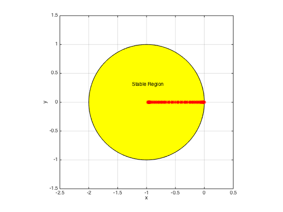
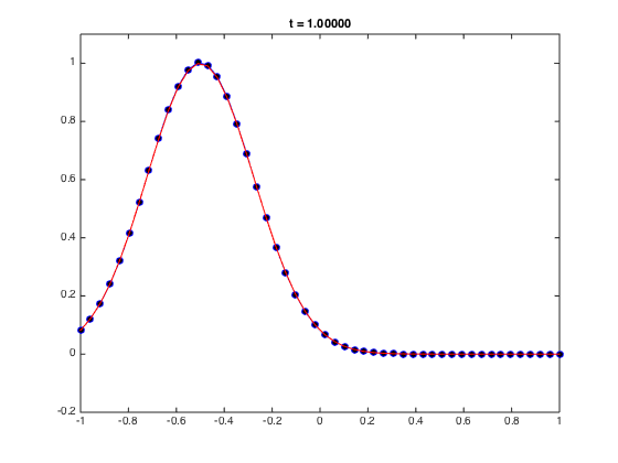
Note that the scaled eigenvalues are in the stability region. Hence, we expect this simulation to be stable. Now let's march the solution in time with Forward Euler.

uexact = @(x,t) exp(-10*((x+t)-0.5).^2);
g1 = @(t) exp(-10*((a+t)-0.5)^2); % Left BC
gn = @(t) exp(-10*((b+t)-0.5)^2); % Right BC
f = @(x,t) -10.*(7+40*t^2-38*x+40.*x.^2+t.*(-38+80*x)).*exp(-10*((x+t)-0.5).^2);

Tinit = 0; Tfinal = 1;
t = Tinit; I = speye(n-2);
u0 = uexact(x,t); % Initial condition
u = u0; u(1) = g1(Tinit); u(end) = gn(Tinit); % Pre-allocate memory to store solution.

figure
graph1 = plot(x,u0,'-ob','markerfacecolor','k'); % Plot of numerical solution
hold on
graph2 = plot(x,u0,'-r'); % Plot of exact solution
t1 = title(sprintf('t = %3.5f',t));
ylim([-0.2 1.1])

while t < Tfinal
    u(2:end-1) = (I + k*D2)*u0(2:end-1) + k*LFCols*[g1(t);gn(t)] + k*f(x(2:end-1),t);
    t = t + k; u(1) = g1(t); u(end) = gn(t); % Update time and boundary values.
    set(graph1,'ydata',u); % update the plot
    set(graph2,'ydata',uexact(x,t)); % update the plot
    set(t1,'String',sprintf('t = %3.5f',t));
    pause(0.01)
    drawnow; % draw the updated plot immediately.
    u0 = u;
end

1-D Advection Equation.

Suppose we are trying to numerically simulate the following 1D advection equation in the domain $[-1,1]$ from time $t = 0$ until time $t = 1$

$u_t = u_x$

with boundary condition

$u(1,t)=0$

and initial condition

$u(x,0)=e^{-60(x-0.5)^2}$

We want to solve it with 3-point stencil finite-difference in space and Backward Euler in time.

close all; clear all;
sigma = 1;

n = 500; % Number of points
a = -1; b = 1; h = (b-a)/(n-1); % Note that n points means n-1 intervals
x = linspace(a,b,n).'; % Discretize the domain with n points.
one = ones(n,1); % create a column vector of size n by 1 of ones
D = spdiags([-one one],[-1 1],n,n);
D(1,1:3) = [-3 4 -1]; D(end,end-2:end) = [1 -4 3]; % Modify first and last row (one-sided weights)
D = (0.5/h)*D; % Don't forget the 1/(2*h) factor

Since $u_n = u(1,t) = 0$ , then the last row and the last columns of D have to be removed (Strip Rows and Columns Method).

D(end,:)=[]; D(:,end)=[];

Plot the the eigenvalues scaled with time-step k of the modified differentiation matrix.

k = h*sigma; % time-step
evscaled = k*eig(full(D));

figure; plot(real(evscaled),imag(evscaled),'*r'); hold on
z = exp(1i*pi*(0:200)/100); r = z-1; s = z; R = r./s;
plot(R); fill(real(R),imag(R),'y')
text(0.5,0,'Unstable Region'); xlabel('x'); ylabel('y')
axis([-2.5 2.5 -2 2]), axis square, grid on

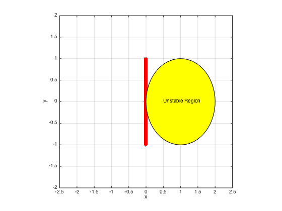
Note that the scaled eigenvalues are always in the stability region. Hence, we expect this simulation to be stable. Now let's march the solution in time with Backward Euler.

uexact = @(x,t) exp(-60*((x+t)-0.5).^2);

Tinit = 0; Tfinal = 1;
t = Tinit; I = speye(n-1);
u0 = uexact(x,t); % Initial condition
u = u0; u(end) = 0; % Pre-allocate memory to store solution.

figure
g1 = plot(x,u0,'-ob','markerfacecolor','k'); % Plot of numerical solution
hold on
g2 = plot(x,u0,'-r'); % Plot of exact solution
t1 = title(sprintf('t = %3.5f',t));
ylim([-0.2 1.1])

while t < Tfinal
    t = t + k;
    u(1:end-1) = (I-k*D)\u0(1:end-1);
    set(g1,'ydata',u); % update the plot
    set(g2,'ydata',uexact(x,t)); % update the plot
    set(t1,'String',sprintf('t = %3.5f',t));
    pause(0.01)
    drawnow; % draw the updated plot immediately.
    u0 = u;
end

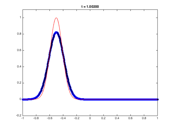
We will discuss why there is a dissipation phenomena in the Advection case.

Published with MATLAB® R2014b