Using Parametric Equations to Shoot Basketballs

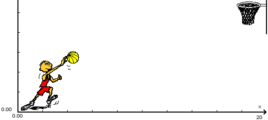
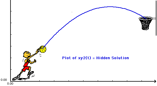
In this "game type" activity, you will use parametric equations to model the trajectory of a basketball being thrown into a basket.

You will need to resize the Graph window to see the entire "basketball" picture. You can drag the window's grow box to make the window larger, or you can specify the size of the Graph window (which is a better way especially if you want the same size window for use in the future).

Select Axes Style... from the Graph menu.
An axes Style window will be displayed.
Enter 500 for the horizontal axis pixel length and enter 400 for the vertical axis pixel length.
Click the OK button.
The Graph window is resized and the entire "basketball" picture is now visible.

Using the equations of motion, the horizontal motion of the ball can be modeled by

x(t) = x0 + v0 cos(a) t

and the vertical motion of the ball can be modeled by

y(t) = y0 + v0 sin(a) t - (1/2) g t^2

where

(x0, y0) = coordinates of the initial position of the ball just before it is thrown (ft)
v0 = velocity with which the ball is thrown (ft/sec)
a = the angle with the horizontal at which the ball is thrown (radians)
g = acceleration due to gravity = 32 ft/sec^2

Note that x0, y0, and g are all fixed. You need to find the values of v0 and a that will give a trajectory that scores a basket.

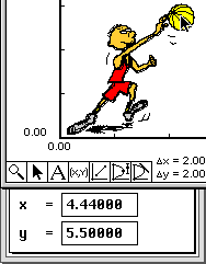
To determine x0 and y0,

Click in the Graph window to make it the active window.
Move the arrow cursor to point to the middle of the basketball. Read the coordinates of the basketball from the "x =" and "y =" cells in the Domain & Range window.

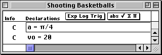
Let's enter a and v0 into the Graph window as constants (parameters of the problem).

Select New Constant from the Work menu.
Delete the default name of the constant in the first row of the Work window and enter "v0 = " followed by the value of your estimate for the initial velocity of the ball. For example, if your estimate for the initial velocity of the ball is 20 ft/sec, then enter v0 = 20 into the first row of the Work window. Press the Enter key.
Select New Constant from the Work menu.
Delete the default name of the constant in the first row of the Work window and enter "a = " followed by the value of your estimate for the angle (radians) at which the ball is thrown. Press the Enter key.

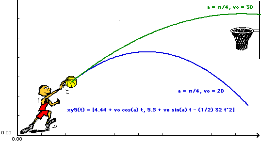
Replace x0, y0, and g by their values in the equations of motion.

Select New Function from the Work menu.
The template xy#(t) = [ , ] is written into the first cell in the Work window.
Enter the x(t) function before the comma and the y(t) function after the comma, that is,
xy#(t) = [x0 + v0 cos(a) t, y0 + v0 sin(a) t - (1/2) g t^2]

(with numbers in place of x0, y0, and g).
Press the Enter key.
Select Plot from the Graph menu.

Did you score a basket? If not,

Change the values of v0 and a.
Select the equations of motion xy#(t) in the Work window.
Select Overlay Plot from the Graph menu.

If your Graph window is the 500 X 400 pixel size, an example basket scoring shot is given by the parametric equations found in the hidden function xy2(t) in the Work window.

Select the hidden function xy2(t) in the Work window.
Select Overlay Plot from the Graph menu.

How does your shot's trajectory compare to the hidden trajectory?

To see the hidden parametric equations,

Select the hidden function xy2(t) in the Work window.
Select Show Hidden Function from the Options menu.

Return to Topic Start

Return to Examples Menu