Taylor Polynomials in Polar Coordinates

Reference: Sheldon P. Gordon, "Taylor Polynomial Approximation in Polar Coordinates" The College Mathematics Journal, Vol. 24, No. 4, September 1993.

This demonstration motivates the study of both Taylor Polynomials and Polar Coordinates. Examples are given that visually demonstrate the convergence of Taylor Polynomials to the classic polar graphs of a circle, cardioid, and four petal rose.

It is well known that the nth degree Taylor polynomial approximation for the sine function in Cartesian coordinates is

sin(x)

x - x^3/3! + x^5/5! - ... +(-1)^(n+1) x^(2n-1)/(2n-1)!

A simple change of variable gives the approximation in Polar coordinates

sin(t)

t - t^3/3! + t^5/5! - ... +(-1)^(n+1) t^(2n-1)/(2n-1)!

Reminder: For this demonstration, the Work window contains a lot of functions. Only five functions can be active (checkmark to the left of the function) at one time. Only active functions can be plotted. Thus, to plot a function that is not active (no checkmark to the left of the function), simply click in the spot where the checkmark should be located and a checkmark will be drawn making the function active and plottable. The checkmark from the "oldest" function will be removed.

The Circle

Plot r1(t) = sin(t) on -/2t/2.
Select the 1st degree Taylor polynomial approximation r2(t) = t in the Work window.
Select Overlay Plot from the Graph menu.
Select the 3rd degree Taylor polynomial approximation r3(t) = t-t^3/3! in the Work window.
Select Overlay Plot from the Graph menu.
Select the 5th degree Taylor polynomial approximation r4(t) = t-t^3/3!+t^5/5! in the Work window.
Select Overlay Plot from the Graph menu.
Note that at least from a visual perspective, the 5th degree Taylor polynomial matches the graph of the polar circle on -/2t/2.

The Cardioid

Plot the cardioid r5(t) = 1 + sin(t) on -t. Note the change in the plotting domain.
Overlay the plot of the 1st degree Taylor polynomial approximation r6(t) = 1+t.
Overlay the plot of the 3rd degree Taylor polynomial approximation r7(t) = 1+t-t^3/3!.
Overlay the plot of the 5th degree Taylor polynomial approximation r8(t) = 1+t-t^3/3!+t^5/5!.
Overlay the plot of the 7th degree Taylor polynomial approximation r9(t) = 1+t-t^3/3!+t^5/5!-t^7/7!.
Overlay the plot of the 9th degree Taylor polynomial approximation r10(t) = 1+t-t^3/3!+t^5/5!-t^7/7!+t^9/9!.

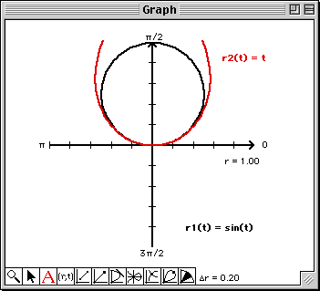
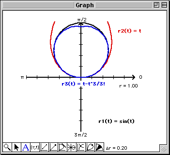
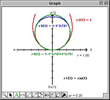
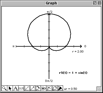
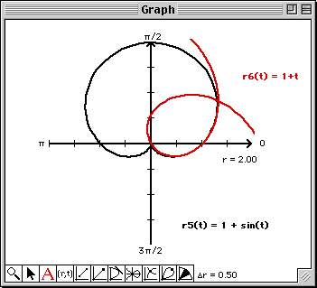
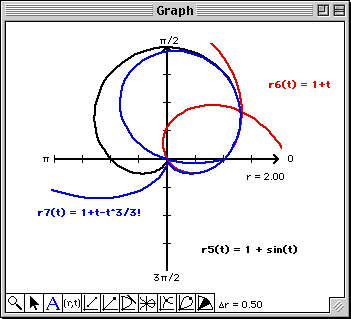
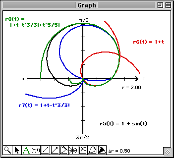
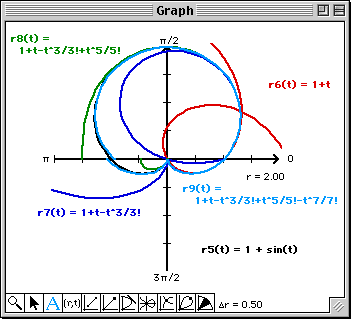
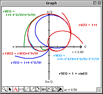
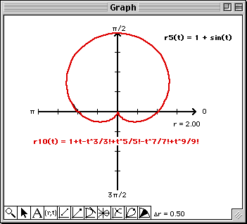
Note that at least from a visual perspective, the 9th degree Taylor polynomial matches the graph of the polar cardioid on -t. Since the Graph window is a bit messy, you can get a better look at the approximation by doing the following:
Plot the cardioid r5(t) = 1 + sin(t) on -t.
Overlay the plot of the 9th degree Taylor polynomial approximation r10(t) = 1+t-t^3/3!+t^5/5!-t^7/7!+t^9/9!.

Plot of cardioid and r10

The Four Petal Rose

Plot r11(t) = sin(2t) on -t.
Select r12(t) = (i,1,1,(-1)^(i+1) (2t)^(2i-1)/(2i-1)!) in the Work window.

This expression represents the nth degree Taylor polynomial in sigma notation, that is, in TEMATH the summation

(-1)^(i+1) (2t)^(2i-1)/(2i-1)!
i=1

is written as

(i, 1, n, (-1)^(i+1) (2t)^(2i-1)/(2i-1)!). Note that the value of n is the third argument.

Overlay the plot of the 1st degree Taylor polynomial approximation r12(t) = (i,1,1,(-1)^(i+1) (2t)^(2i-1)/(2i-1)!).
Change the third argument in r12(t) from "1" to "2", that is, r12(t) = (i,1,2 ,(-1)^(i+1) (2t)^(2i-1)/(2i-1)!).
Overlay the plot of the 3rd degree Taylor polynomial approximation r12(t) = (i,1,2,(-1)^(i+1) (2t)^(2i-1)/(2i-1)!).
Continue to increase the degree of the approximating Taylor polynomial by editing r12(t) and overlaying the plot of the new polynomial until the plot of the polynomial matches the plot of the four petal rose.

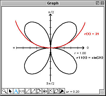
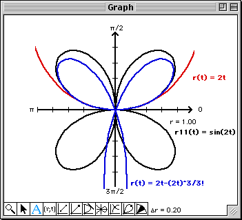
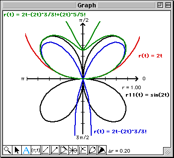
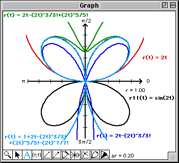
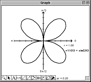
The Graph window will soon become quite messy. To visualize each approximation a bit better, click on the vertical line to the left of r12(t) to change the color of the plot each time you edit r12(t). When the Graph window gets real messy, simply plot r11(t). This will clear the Graph window and plot the four petal rose. You can now continue overlaying the higher order polynomial approximations.

Return to Topic Start

Return to Examples Menu