Using a Logarithmic Spiral to Model a Chambered Nautilus Shell

Caution: TEMATH's tools will write the values of computed results at the bottom of this Report window. This will cause you to constantly scroll between the computed results and the instructions for this activity. You may want to print a copy of the contents of the Report window before you begin this activity.

We used a digital camera to take a picture of a Chambered Nautilus shell. We downloaded the picture into our computer and used a picture viewing software package to display the picture. Using copy and paste, we copied the picture and pasted it on top of the axes plotted in TEMATH's Graph window. Using TEMATH's Selection tool on the tool palette and the arrow keys on the keyboard, we repositioned the picture so that the center of the spiral was located at the origin (pole). To see the entire shell picture,

Select Axes Style... from the Graph window.
Set the horizontal axis pixel length to 500, set the vertical axis pixel length to 500.
Click the OK button.

We will use Polar Coordinates and the logarithmic spiral

bt
r = a e

to model the spiral of the Chambered Nautilus shell.

In the first part of this activity, we will show you an example spiral fit to the shell and in the second part, we will give you directions for finding your own spiral fit.

Select Overlay Plot from the Graph menu.
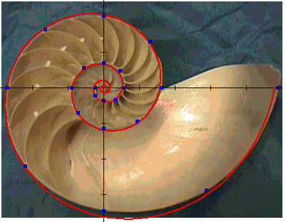
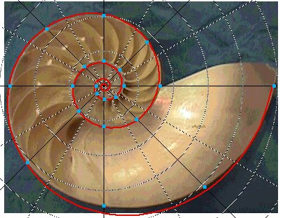
The points that we sampled along the spiral of the Nautilus shell are plotted on top of the picture of the shell.
Select spiral(t) in the Work window.
Select Overlay Plot from the Graph menu.
The "Least Squares" logarithmic spiral fit is plotted on top of the picture of the shell. Note how well you can mathematically model nature.

To find your own spiral fit, follow these directions.

Select Plot Axes from the Graph menu. This erases our example data and fit.
Select Grid from the Graph menu.
Click the Coordinate (Point) tool on the Tool Palette.
Click the tool's pop-up menu and select the smallest solid circle point pattern.
Select Color - Red from the Options menu.

You are now set to click (sample) points along the shell's spiral at increments of

/4 (45°).

Position the "Plus" cursor over the part of the spiral that crosses the left half of the horizontal axis closest to the origin (at approximately r = 0.6 and t = ).
Click the mouse button and a point will be drawn. Use this point away from the origin as your first sampled point since the spiral is too small closer to the origin to get any sampling accuracy.
Continue in a counterclockwise direction along the spiral and click a point every /4 (45°) radians. Use the grid lines for reference. You should click a total of 21 points.
Select Generate Table from Points from the Tools menu.

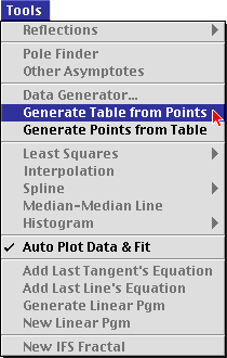
The coordinates of the points drawn in the Graph window will be stored in a data table written into the top cell of the Work window.

The next step is to find the least squares natural exponential fit to the data. We must copy the data from Polar Plot mode to Cartesian (Rectangular) Plot mode to find the fit.

Select Show Data Table from the Work menu.
The Data Table window is opened and the data is displayed.
Select Select Data Table from the Edit menu.
Select Copy from the Edit menu.
Click the close box of the Data Table window. This closes the window.
Select Rectangular from the Graph menu.
Select New Data Table... from the Work menu.
Double-click the Resize command located in the Data Table's list of commands.
Type 21 into the command area located at the top right of the Data Table window.
Press the Enter key or click the enter button.
Position the cursor over the C1 column label.
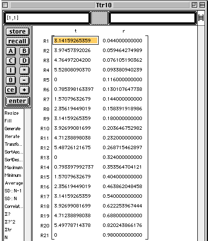
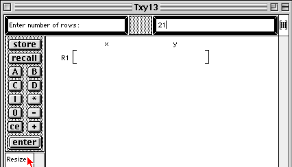
The cursor changes to a downward-pointing arrow.
Press and hold down the mouse button. Drag to the right until both columns are selected.
Select Paste from the Edit menu.
The values of the data are pasted into the table.

Notice the first column of values. These are the values representing the t (angle) coordinate of the clicked points. Note that they are all between 0 and 2

. Thus, we must adjust them for the increasing angle of the spiral.

Position the cursor over the x column label.
The cursor changes to a downward-pointing arrow.
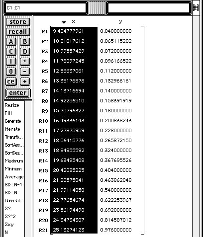
Click the mouse button to select the first column.
Double-click the Fill command located in the Data Table's list of commands.
The fill function template "x(i) = ?" is displayed in the command area.

In order to find a fit, the first coordinates must represent the increasing t-values of the spiral. Thus, we must replace the points' first coordinates with an increasing sequence of values that differ by a multiple of 2

from the original values. For example, since we sampled our first point at t = 3

and continued in increments of

/4, we will use the sequence of t-values

, 3

/4, ...., 3

+ (

/4)(i-1),....

Type the following fill function into the command area: x(i) = 3+(/4)(i-1) The variable i represents the row number of the data table.
Press the Enter key or click the enter button.
The first column is filled with the angles that we need.
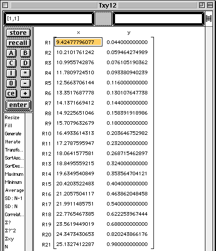
Select Add Data Table from the Work window.
The data table will be added to the Work window.
Select Plot from the Graph menu.
Select Least Squares - Natural Exponential from the Tools menu.
The least squares natural exponential fit is drawn in the Graph window and its algebraic expression is written into the top cell of the Work window.
Click in the Work window and select the portion of the algebraic expression of the least squares natural exponential fit that is to the right of the equal sign.
Select Copy from the Edit menu.

The next step is to copy the least squares natural exponential fit to the Polar Plot mode.

Select Polar from the Graph menu.
Select New Function from the Work menu.
Select Paste from the Edit menu.
The expression for the least squares natural exponential fit is pasted into the top cell of the Work window.
Select the variable x in the expression and replace it with the variable t (t is the independent variable in Polar Plot Mode). Press the Enter key.
Select Plot from the Graph menu.
Your fit along with the picture of the shell is drawn in the Graph window.
Select your data table in the Work window.
Select Overlay Plot from the Graph menu.

Return to Topic Start

Return to Examples Menu